The tools consist of two main parts. The first part runs in QGIS, the second in Rhino Grasshopper.

The current version (0.3.x) has been tested and runs on Rhino 7 and QGIS 3.22 (LTR) on Windows 10 and MacOS (Intel/Rosetta).

Step 1:

First you should download Rhino from here, and QGIS 3 from here. We recommend the current the Long Term Release. On Windows, we recommend you choose the Standalone installer.

Note (March 2023): please use the latest 3.22.16 version while we update the software to the new 3.28 LTR. Download here for Mac: QGIS 3.22, and here for Windows. We do not currently have an installer for Linux. Please contact us if this is something you are interested in. 

Mac: Install QGIS by dragging it to your Applications folder. The first time you run it you may need to right click and press open on the dialog to bypass the Mac security measures.

Windows: Install QGIS by running the installer with default options.

Step 2:

Download the QGIS python codes by going to the Tools page and clicking on “Download Triangulation Tools”. Do not unzip the file.

Windows users: If you are running Windows with the default security options, please open QGIS as an administrator in order to install the plugin (right click on QGIS, select ‘run as administrator’).

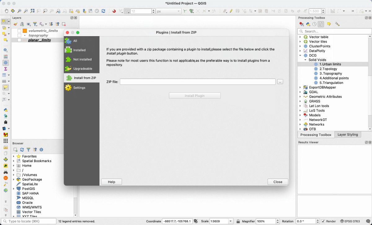
Windows and Mac: Install the CSV plugin by opening QGIS and going to: ‘Plugins’ menu, ‘Manage and Install Plugins’, ‘Install from ZIP’, and choosing your zip file and clicking ‘Install Plugin’. If QGIS asks to install other plugins, please allow. The installation process should be quick, but if you are running QGIS on MacOS older than Big Sur, it can take up to  5 minutes. Important: Wait for the success message bar to show before closing the plugin manager.

Once installed, we recommend you restart QGIS. The plugin will be available in the Plugins menu bar (DCG CSV), or the Processing Toolbox.

Step 3:

The second part of the code runs in grasshopper. Download the script from ‘Download Convex Solids Tool’ in the Tools page. Unzip the file you downloaded. The archive contains an install.gh file, used only once for installation of python dependencies, an import_shapefile.gh file, used to import your particular geometries into Rhino, and a CSV_x_y.gh file, containing the analytical algorithms.

Install Rhino through the usual means for your OS.

Windows users: If you are running Windows with the default security options, please open Rhino as an administrator in order to install the plugin (right click on Rhino, select ‘run as administrator’).

Open Grasshopper (type grasshopper in the Rhino command line) and while in Grasshopper, open the install.gh script inside the folder you just unzipped. Double click on the Install toggle button to begin the installation process. Once it is finished, you can close grasshopper, shut down Rhino, and delete the install.gh file.

You can now open Rhino and Grasshopper, and open the CSV script. The first time you run it, it may ask to install a few plugins. Let it. You can now follow the rest of the tutorial.

1. Preparation.

First you need to prepare your geometry in Rhino. If you don’t already have 3D geometry of the area you will analyze in Rhino, one way to acquire 3d urban geometry is to import it from GIS files using a plugin such as Heron or BearGIS (both available from the Rhino Package Manager).

In the near future the Solid Voids Toolset will import shapefiles directly for analysis. For now please use the import_shapefile.gh grasshopper code we provide along with the toolset as described below.

2. Buildings and walls.

Simply select your shapefile on the left and turn the toggle to ‘True’. The Elevation Index value should correspond to the column number where height information for the building polygons are located (this can be seen in the ‘flds’ panel). At the end of the process, you may bake the buildings. For walls, the process is the same, but take care to alternate the ‘C’ switch of the Polyline component between ‘open’ and ‘closed’ depending on whether the wall geometries are open linestrings or closed polygons.

2. Topography and terrain.

Simply select your shapefile on the left and turn the toggle to ‘True’. As before, the Elevation Index value should correspond to the column number where height information for the topography points are located (this can be seen in the ‘flds’ panel). If you wish to experiment with the mesh smoothing values, you may use the ‘Contour’ component in the ‘Visualise’ group (next image) to more effectively check the effects on the terrain. At the end of the process, you may bake the terrain.

3. Interpolated topography points.

This group subdivides the mesh into equal squares. Simply choose the degree of interpolation in the ‘Size’ component. Once you are happy with the level of detail, you may bake the interpolated points.

4. Error checks.

The above process will allow you to input most geometry for analysis with little adaptation. Once imported however, it is necessary to check the geometry within the Rhino canvas window to confirm that all buildings are of sufficient height and above the terrain. When this is not the case, you will need to correct either the building height or the terrain. All analysis (including QGIS algorithms) uses the 3D geometry in Rhino – there is no need to correct the original shapefiles unless you wish to.

Below we list the necessary geometry and what you need to pay attention to while creating it:

• Buildings: these need to be extrusions of flat polygons on the XY plane. Their base should not sit on top of the topography mesh, but the XY plane, at Z=0.
• Walls: these are boundaries that you usually have to model manually, unless you already have a detailed GIS file or a 3d model. The walls should be extrusions of line geometry sitting on the XY plane, and not the topography mesh, just like the building geometry. This is why, all boundaries will essentially be modeled like walls, may they be hedges, fences, gates, removable parking barriers or in some cases, parking lots. You should decide if the urban space they separate is accessible or not, and accordingly model the barrier or not. Below are several cases of boundaries that may be modeled as walls.

• The topography mesh: the code only requires topography points (located at their correct elevations). Nevertheless, it is advisable to first create a delaunay mesh and make sure that the top-most vertices of the walls and building geometry remain above the mesh geometry (avoid the case in the image below). Otherwise, the QGIS code will give you an error. If the topography points are not dense enough, you may also get an error in the 3rd QGIS code you are going to run in the next step. If that happens, extrapolate a denser set of topography points. For this, you can project a 10m x 10m grid of points on the delaunay mesh.

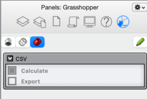
Once you have your geometry ready, open the grasshopper file. Once it finishes loading you can minimise the grasshopper window and use the Grasshopper panel in Rhino (right click on the panel and select Grasshopper if it’s not active. There are only two options: Calculate and Export. Press on Calculate to open the CSV Solution calculation window.

The CSV Solution window is where all the options and calculations take place. It is divided into eight tabs:

• Pj (CRS projection)
• Ot (geometry out)
• In (geometry in)
• CS (calculate convex spaces)
• CV (calculate convex voids)
• SV (calculate solid voids)
• Fc (visualise facades)
• Fl (visualise flows)

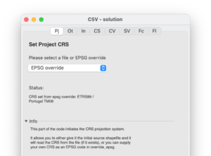
The window should open with the Pj (Projection) tab active. If not, select it. In this part, you will define the CRS that will be used throughout your project. You can either obtain it by reading from an existing shapefile .prj file, or you can attribute an EPSG code by selecting EPSG override. The script accepts most EPSG codes. In this example we enter 3763, for EPSG:3763 used in Portugal mainland. If successful, the status message will inform you of the CRS selected and you can continue with the next step.

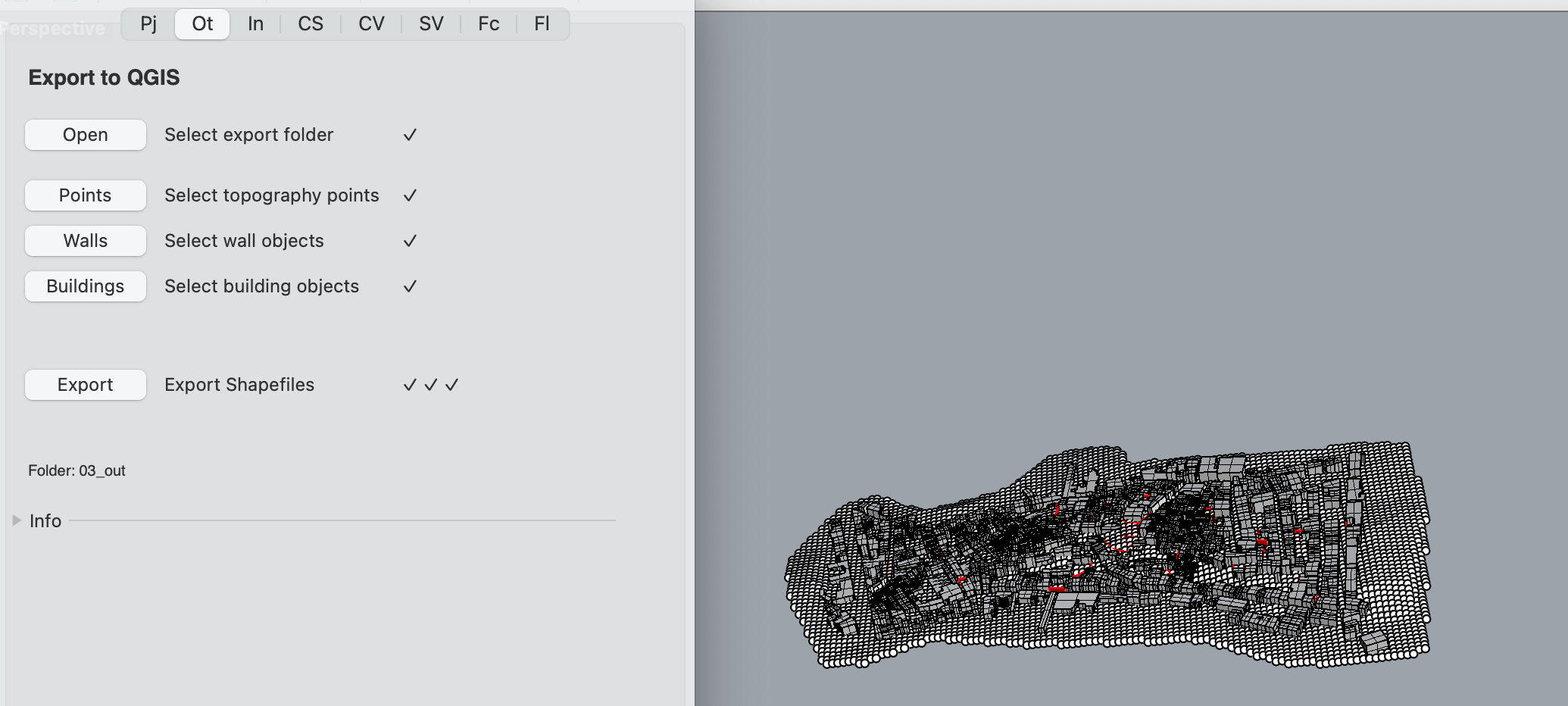
In this step, we select the Ot (output) tab to convert the rhino geometry to ESRI shapefiles. We need topography points,* building volumes (3D polygon BREPS representing buildings), other urban limit volumes (vertical planar BREP elements that represent all physical barriers such as gates, walls, hedges etc.), and if there is a shoreline, a polygon defining the water limit.* If the topography points are not sufficiently dense (please see screenshot), consider creating more through extrapolation (see Step 1 –  Preparing the geometry).

We simply select the output folder to be used to export all the files, and then proceed to select the topography points, walls, and buildings, by clicking on the relevant button to activate the Rhino selection tool. Once all the selections have been made we click on export and wait for the process to finish.

* Water and other horizontal limits are still under development and not available at this time.

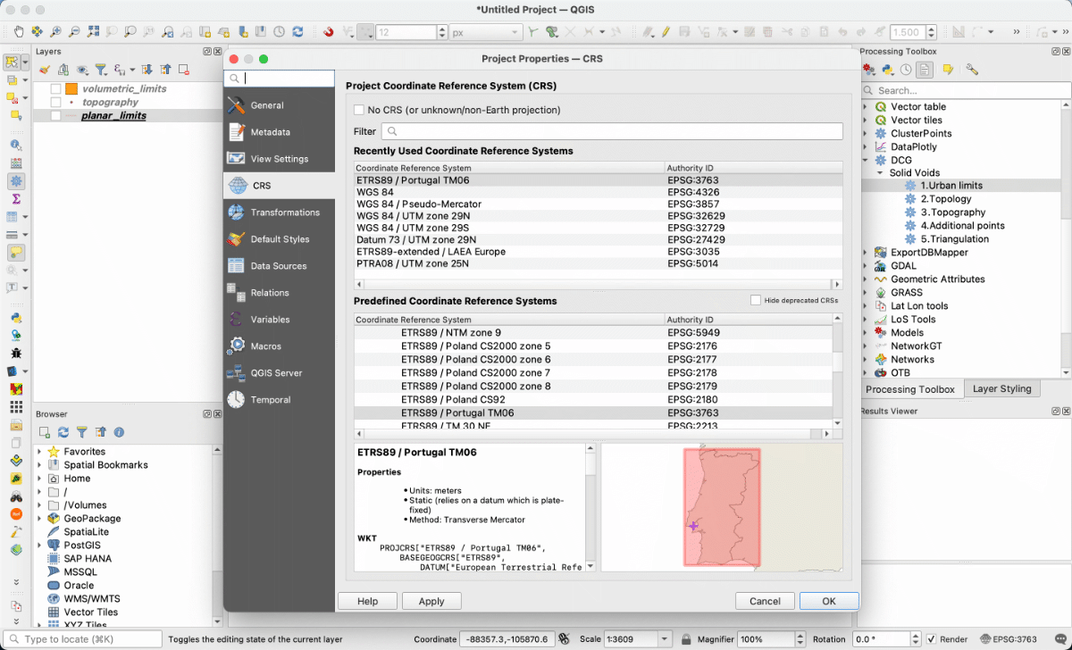
1- Prepare the QGIS working CRS: Always remember to use the correct CRS for your site. For our tutorial, we will be working will Lisbon data which carries the standard Lisbon CRS known as ETRS89 / Portugal TM06 (EPSG:3763). Please make sure QGIS OTF (on the fly transformation) is activated and set to a CRS of EPSG:3763. Whenever you add a file from grasshopper to the project, take a moment to confirm it has the correct CRS. Likewise, whenever you run a script in QGIS, confirm the resulting file has a CRS attached before exporting it. You can define the project CRS by clicking on the bottom right main window globe or by selecting menu item ‘Project -> Properties’. You can define a layer with a known missing CRS through the Processing Toolbox or by right clicking on the layer and selecting ‘Properties’. Do not change the CRS of a layer with a valid coordinate reference system attached (in this case you should re-project it).

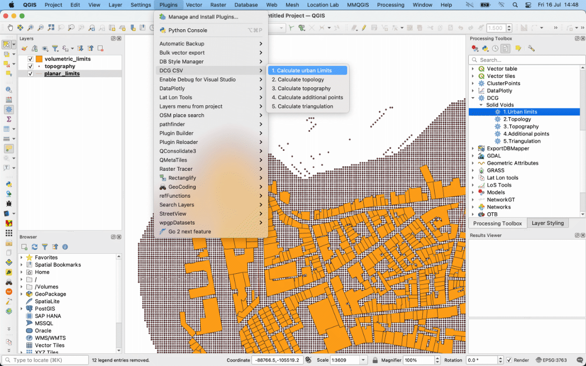
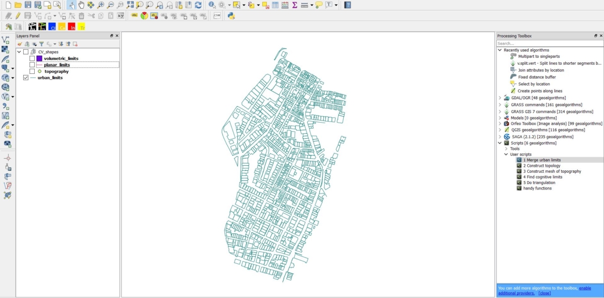
2- Import all shape files generated in the first step to QGIS: volumetric limits, planar limits and topography. The CSV algorithms can be accessed either from the plugins menu, under ‘DCG CSV’, or from the Processing Toolbox, under ‘DCG – Solid Voids’.

3- Run the first code: “Merge Urban Limits.” This code receives volumetric limits and planar limits as input. “There are no horizontal limits” checkbox should be checked at this stage as no horizontal limits are generated in the grasshopper code yet.

Do no assign an output file or directory. Simply let the algorithm save the generated files as temporary layers with their default names for now. We will export them all later. Do the same for all five algorithms. You may leave the settings of all algorithms at their default values (please ignore the values in the screenshots).

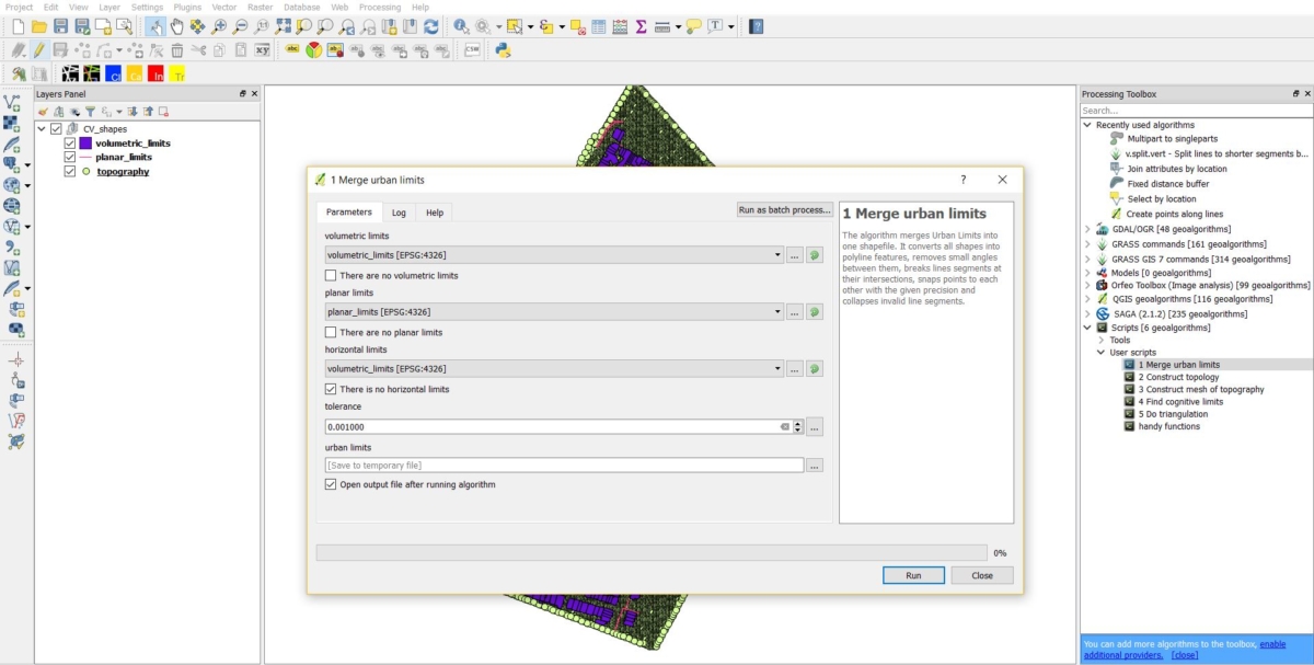
The output of this code will be “urban limits”.

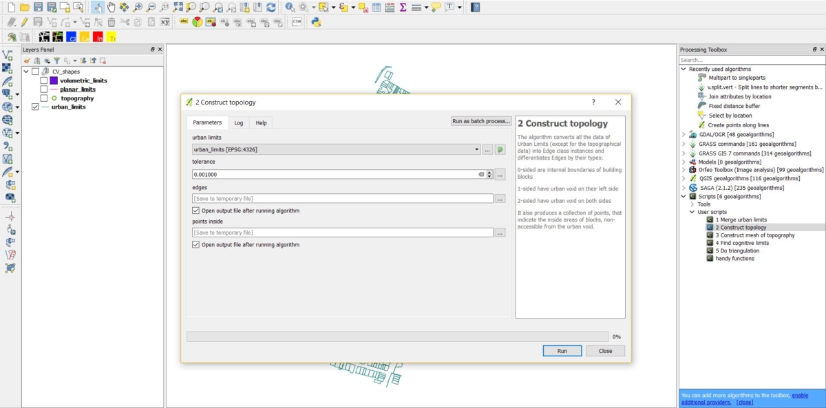
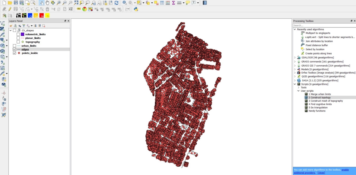
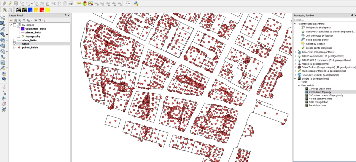
4- Run the second code: “Construct topology.” This code receives “urban limits” as input and creates “points inside” and “edges” as output.

– If you get the error: “not sufficient topography points” do not run the following codes as the final code will not produce geometry after this error. Instead make sure the following issues are resolved and re-run the third code.

• If the topography mesh remains above the upper vertices of any of the urban limits or planar limits at any point, this should be corrected.
• If any geometry extends beyond that of the limits of topography points in plan, the region covered by the topography points should be extended.
• If the error repeats, the topography points may not be dense enough. In this case, a more dense grid of topography points should be generated though extrapolation.

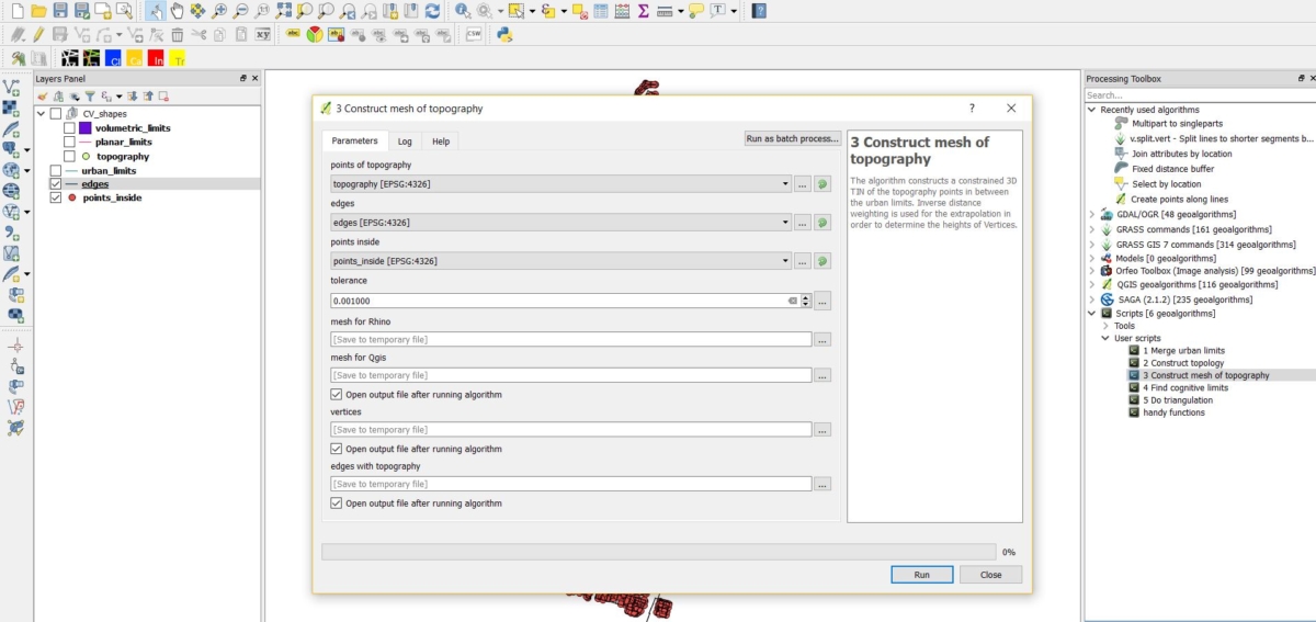
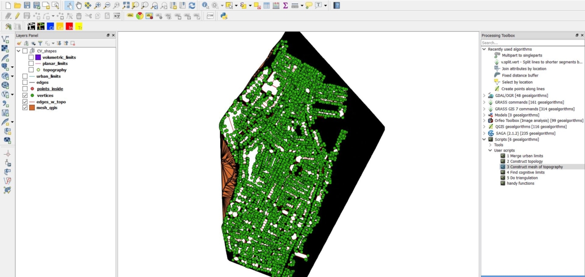
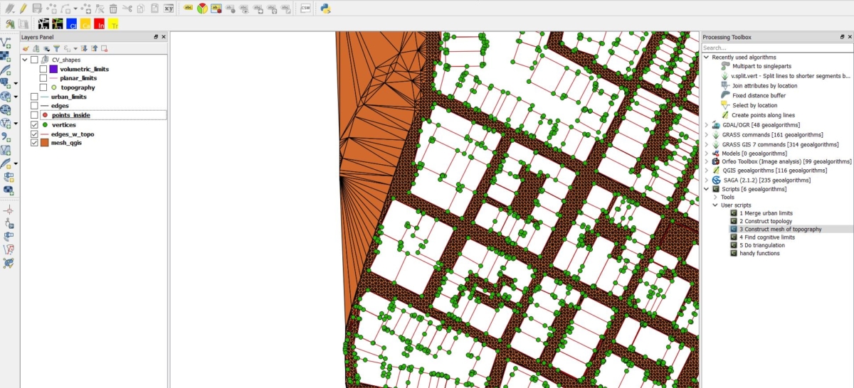
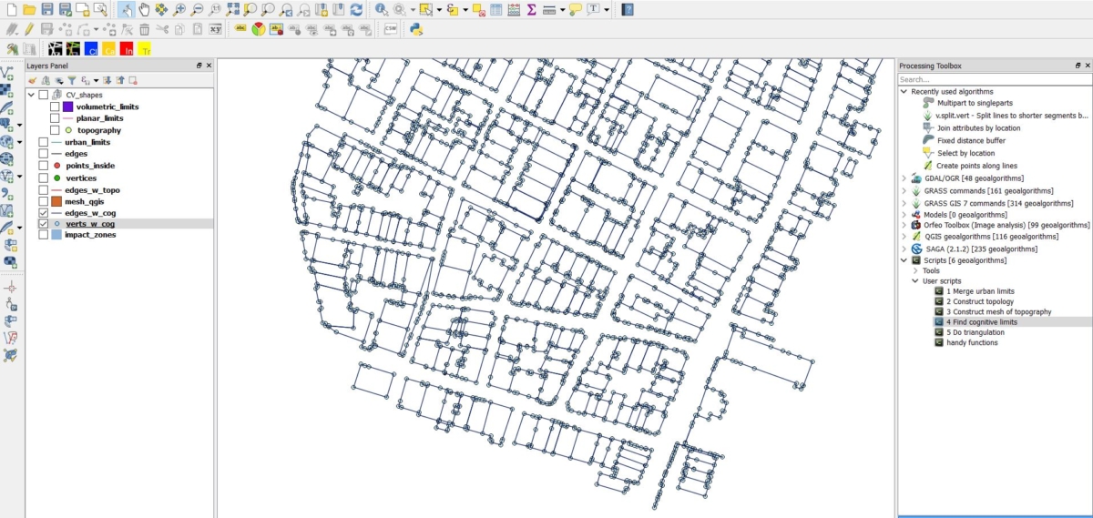
5- Run the third code: “Construct mesh of topography.” This code receives “topography points”, “edges” and “points inside” as input and creates “mesh for qgis”, “vertices”, “edges with topogrpahy.” It also creates a mesh file to be used in the grasshopper code later. This mesh is a .txt file for Rhino. Please save it in your final output folder with the name rhino_mesh.txt.

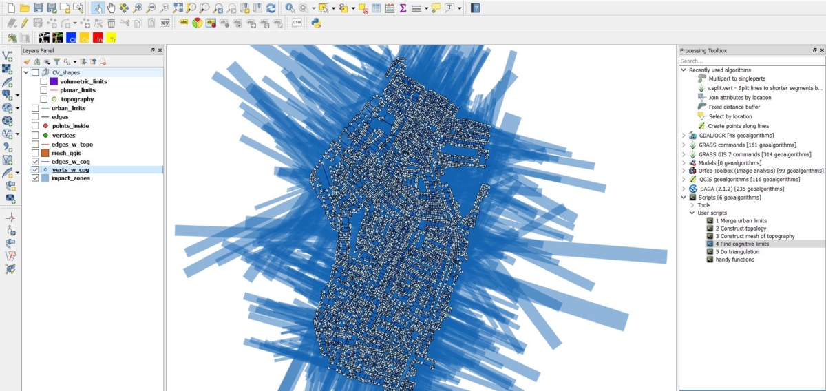
6- Run the fourth code: “Find cognitive limits.” This code receives “edges with topography” and “vertices” as input. The parameters advisable for use for this code are as follows:

• projection parameters:  max(LENGTHx15.0,HEIGHTx1.0,UNITSx5.0);;BEARINGorHEIGHTDIFF
• significant vertex bearing: 30.000000
• significant edge height difference per vertex : 3.000000
• tolerance for vertex proximity: 3.000000

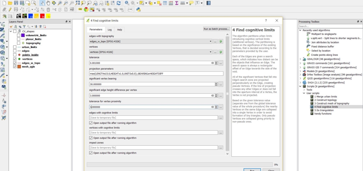
This code defines the implicit limits.

• Search Space: The maximum distance in which implicit points (vertices) should be searched for.
• Attribute of significance: The Significance Precondition of explicit limits to get projected as implicit ones, defined through the bearing angle, vertices’ height difference and vertices minimum horizontal distance.
• When (1) and (2) are satisfied the Explicit limits are projected as Implicit vertices.

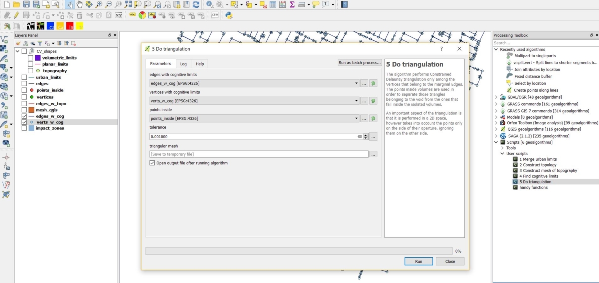
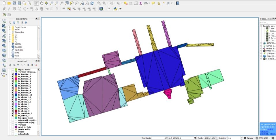
7- Run the fifth code: ” Do triangulation.” This code receives “edges with cognitive limits”, “vertices with cognitive limits” and “points inside” as input and creates the “triangular mesh.”

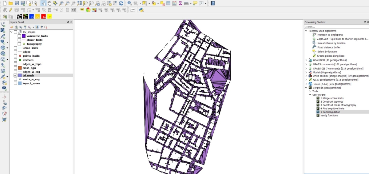
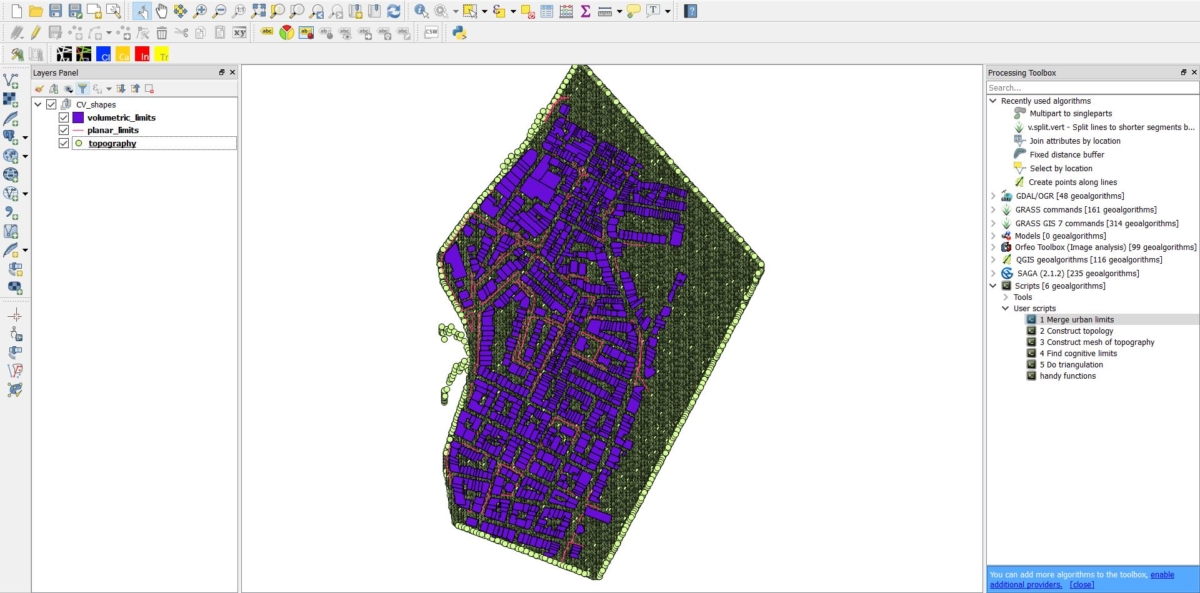
8- Split the mesh: To feed this triangular mesh into the grasshopper definition, it needs to be broken up into smaller meshes. This division needs to be done manually but natural divisible limits of convex spaces should be taken into consideration.

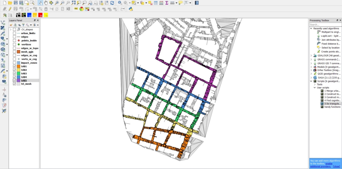
Below is an example demonstrating this division from a different urban context.

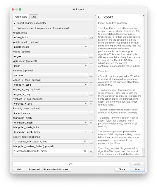
9- Bulk export the layers: Once everything is done, you will have a large number of temporary layers in the layers panel. To save them for future reference and continue the analysis in Rhino, run the sixth code ‘6. Export’. This will export all the layers into shapefiles. You can choose the export location for the files (by default these are placed in a folder on your desktop). The layers are automatically chosen according to their default naming structure – you will need to select them if you used a different structure. If you manually split the triangular mesh, the sub-meshes will all need to be exported as well. You can use a plugin such as ‘bulkvectorexport’ which can export all visible layers in one go. An option is available which will split and export the main triangular mesh – at the moment it is still experimental and we only recommend its usage for the analysis of extremely large urban areas.

1- Back in Rhino, we now load the geometry and data generated in QGIS.

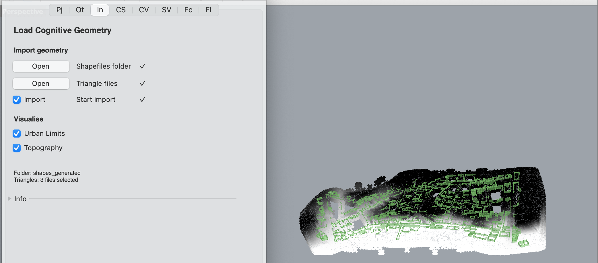
Switch to the In tab and select the folder where the cognitive geometry generated in QGIS was exported. Next, select the trianged mesh within that folder. If the study area is quite large we recommend selecting a limited number of meshes rather than the entire mesh and run the calculations on particular areas first. Click Import and wait for the process to finish.

Once the files have finished importing, you can preview and assess the geometry through the relevant options in the Visualise section of the tab.

2- We can now move on to calculating the Convex Spaces by switching to the CS tab.

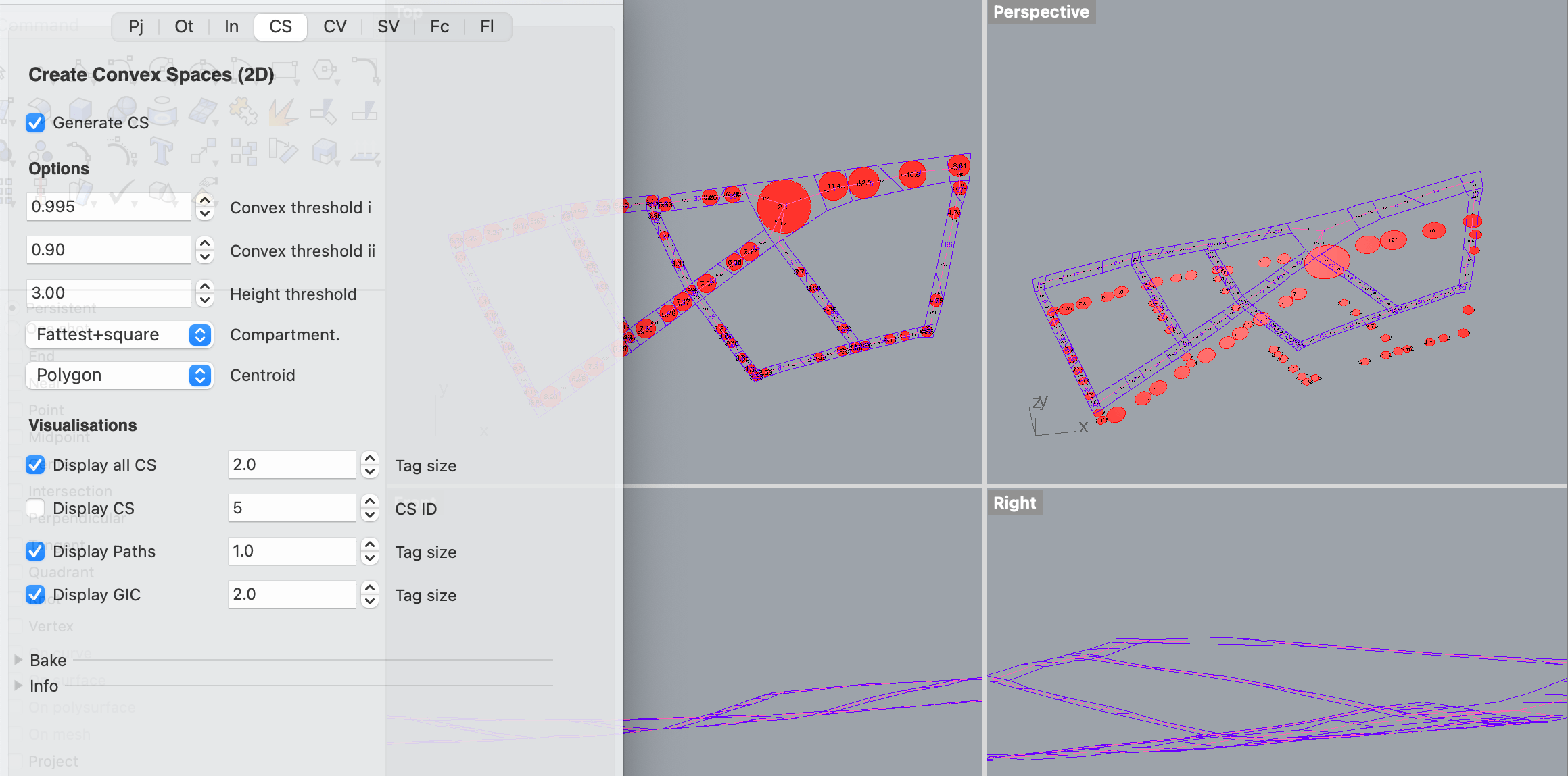
The tab opens with the default options. Whilst we prepare a manual of all the different options, their meanings and definitions can be viewed in the papers published so far. Click on Generate CS to perform the calculation (warning: this is a computationally intensive process that may take some time). Once the calculation is finished, the totality of the convex spaces (CS), individual convex spaces, paths, and greatest inscribed circles (GIC) can be previewed by clicking on the relevant options in the Visualisations section of the tab.

3-  The next step involves generating what we term Convex Voids, by switching to the CV tab.

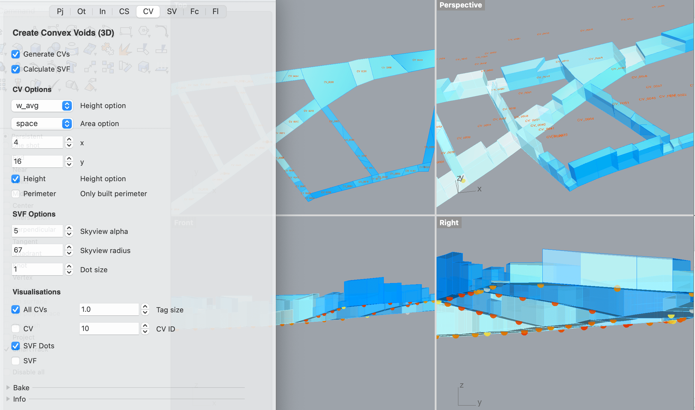
The tab will open with default options. Information on these options can be viewed in the papers published. Make sure the Height option is selected. Click on Generate CVs to proceed with the calculation. Once it finishes, the totality of the convex voids and specific convex voids can be previewed by selecting the relevant options in the Visualisations section of the tab.

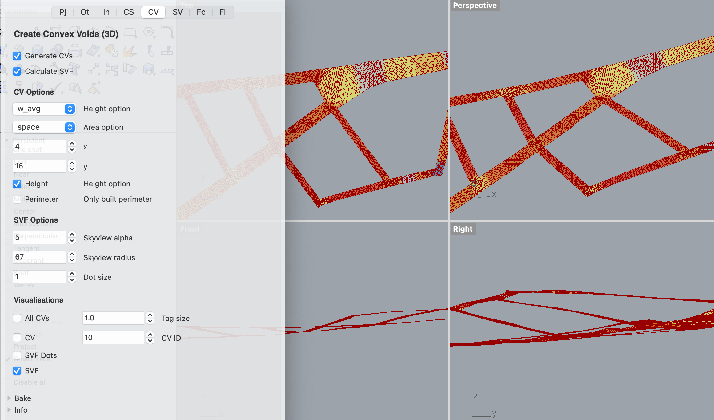
The Sky View Factor (SVF) can also be calculated within this tab. Simply click on Calculate SVF and wait for the process to finish. The output can be previewed by selecting the relevant options within the Visualisations section of the tab.

If you wish, you can expand the Bake section of the tab to bake the previews into permanent Rhino geometry in particular layers. This can also be done for all or particular geometries at the very end of the process by opening the CSV Export window of the Grasshopper panel.

3-  The final calculation involves generating what we term Solid Voids (SVs), by switching to the SV tab.

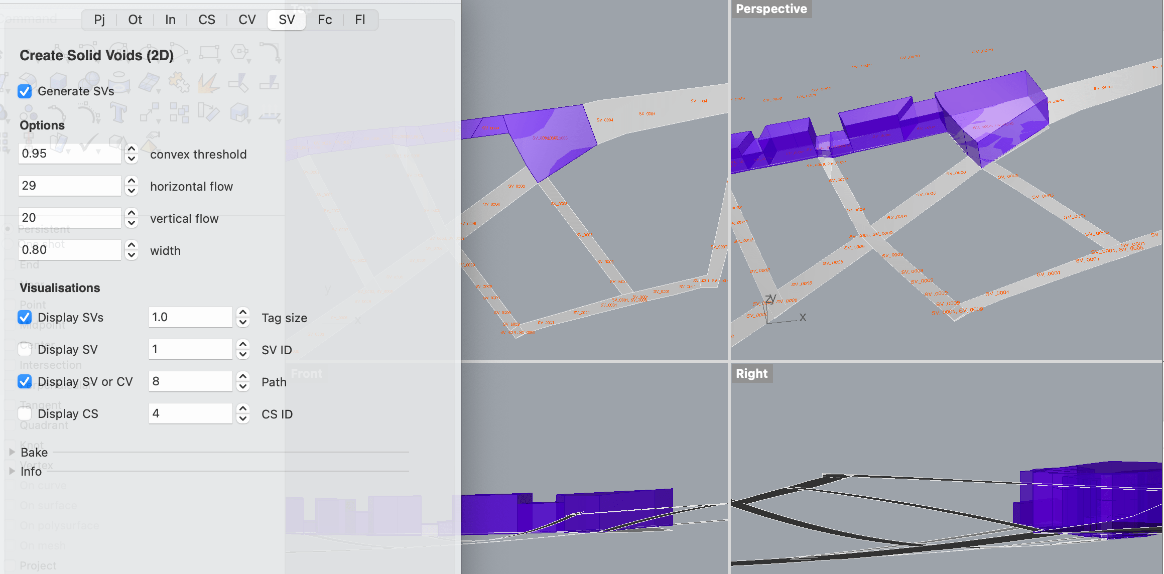
The tab opens with the default options. Information on these options can be viewed in the papers published. Click on Generate SVs to proceed with the calculation and wait for the process to finish.

The totality of the solid voids, particular solid voids, and particular convex voids and convex spaces can be previewed by selecting the relevant options within the Visualisations section of the tab.

If you wish, you can expand the Bake section of the tab to bake the previews into permanent Rhino geometry in particular layers. This can also be done for all or particular geometries at the very end of the process by opening the CSV Export window of the Grasshopper panel.

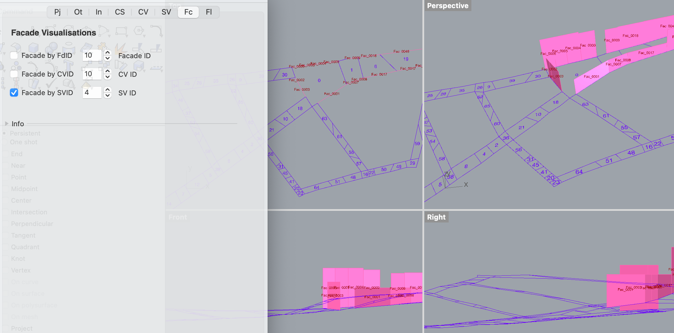
4- Facades and their relation to the voids and convex spaces can be visualised in the Fc tab.

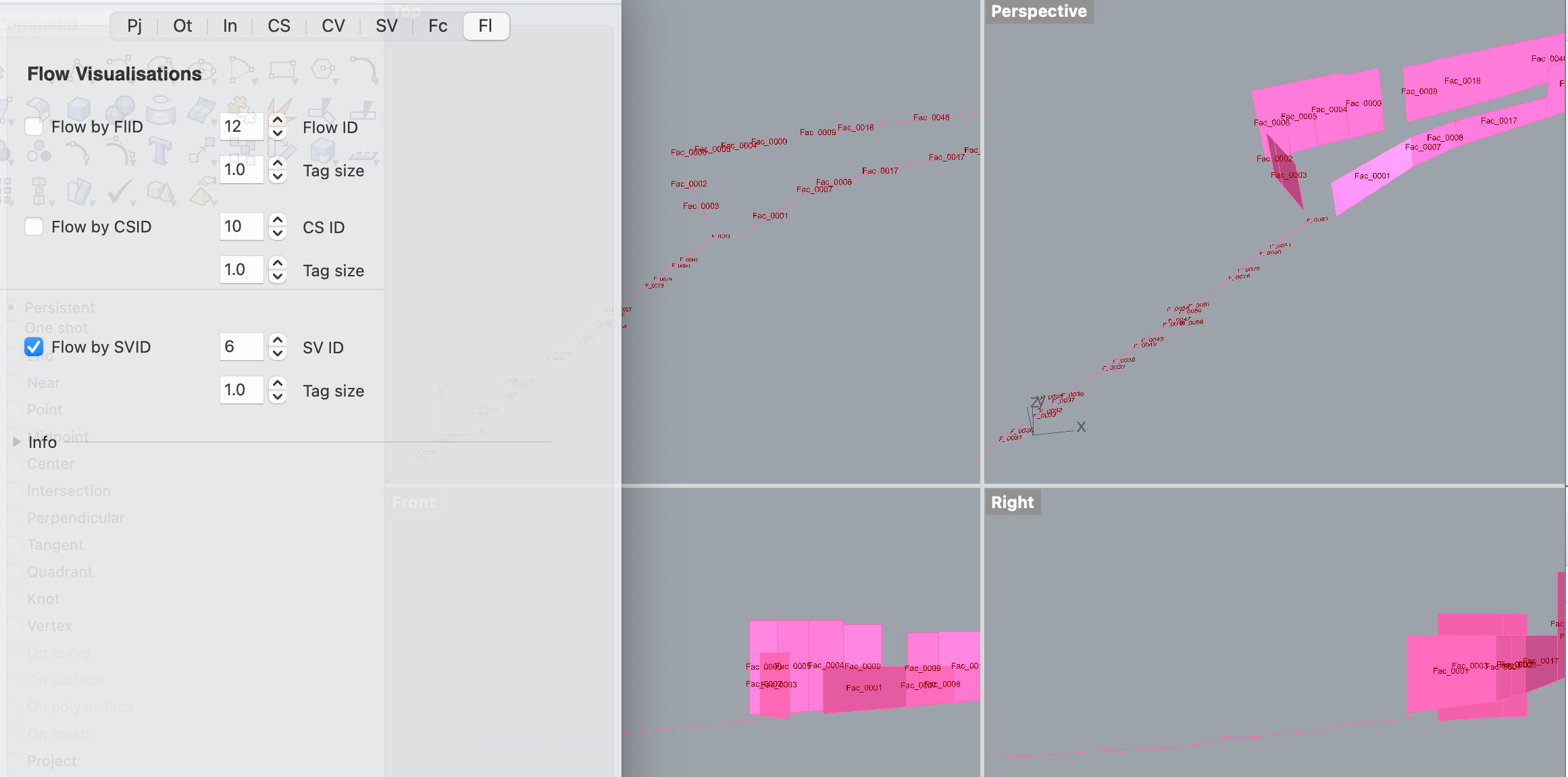
5- Flows and their relation to the voids and convex spaces can be visualised in the Fl tab.

6- Once all the calculations are complete, you can close the CSV Calculate window and open the Export window by clicking on the relevant option in the Grasshopper panel in Rhino.

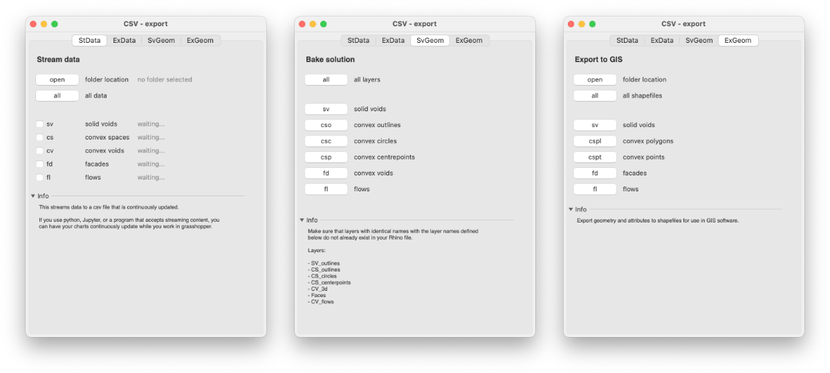
The window is split into four tabs:

• StData (stream data)
• ExData (export data)
• SvGeom (bake solutions)
• ExGeom (export to ESRI shape files)

StData allows you to stream the data generated by the calculations for external real-time analysis. ExData allows you write the final generated data into csv files to import into Excel. SvGeom allows you to bake all or parts of the geometry into the Rhino file. ExGeom allows you to export the geometry and data attributes into shapefiles for use in GIS software.

In the future, we will be providing Jupyter notebooks for real-time analytics and statistical visualisation of the streamed data, as well as integrating a select number of data visualisations within the grasshopper code, allowing you to make changes in any part of the process and have them propagate all the way to the final report building section. Various additional information can be generated using the CS, CV, SV, Facade and Flow data and geometry. Refer to the about page and publications to learn more about the theory and applications of the method.

Convex and Solid Voids is in active development. We are aware of certain errors that may occur and will strive to fix them as soon as we can.

1- If the QGIS plugin does not install properly, or you do not see the algorithms in the menus or Processing Toolbox after installation, this is normally due to restrictive security settings in certain Windows systems. Please uninstall the plugin and quit QGIS. Open QGIS ‘as an administrator’. You should now be able to install the plugin correctly.

2- If the QGIS algorithms fail with an error stating something such as “Algorithm grass7:v.generalize no found”, this means that your GRASS provider is disabled. This has been known to occur in new Windows installs of QGIS. Simply open the Plugin Manager and search for ‘grass’. Make sure that ‘GRASS GIS provider’ is enabled.

3- If the QGIS algorithms fail with an error stating something ending with “.gpkg not found”, this means that QGIS was not able to write its temporary files to the system. This has been known to happen in Windows Home systems with non-ASCII characters in the user folder or restrictive security settings. This is an upstream issue with QGIS – we are investigating possible solutions.

4- If you notice issues or failures while running the analysis in Grasshopper / Rhino, most of the time this is due to inadequate splitting of the main triangular mesh. Please confirm that each shapefile of the triangular mesh consists of a continuous mesh, and that there are no duplicate polylines when all layers are compared together.