
1- Back in Rhino, we now load the geometry and data generated in QGIS.
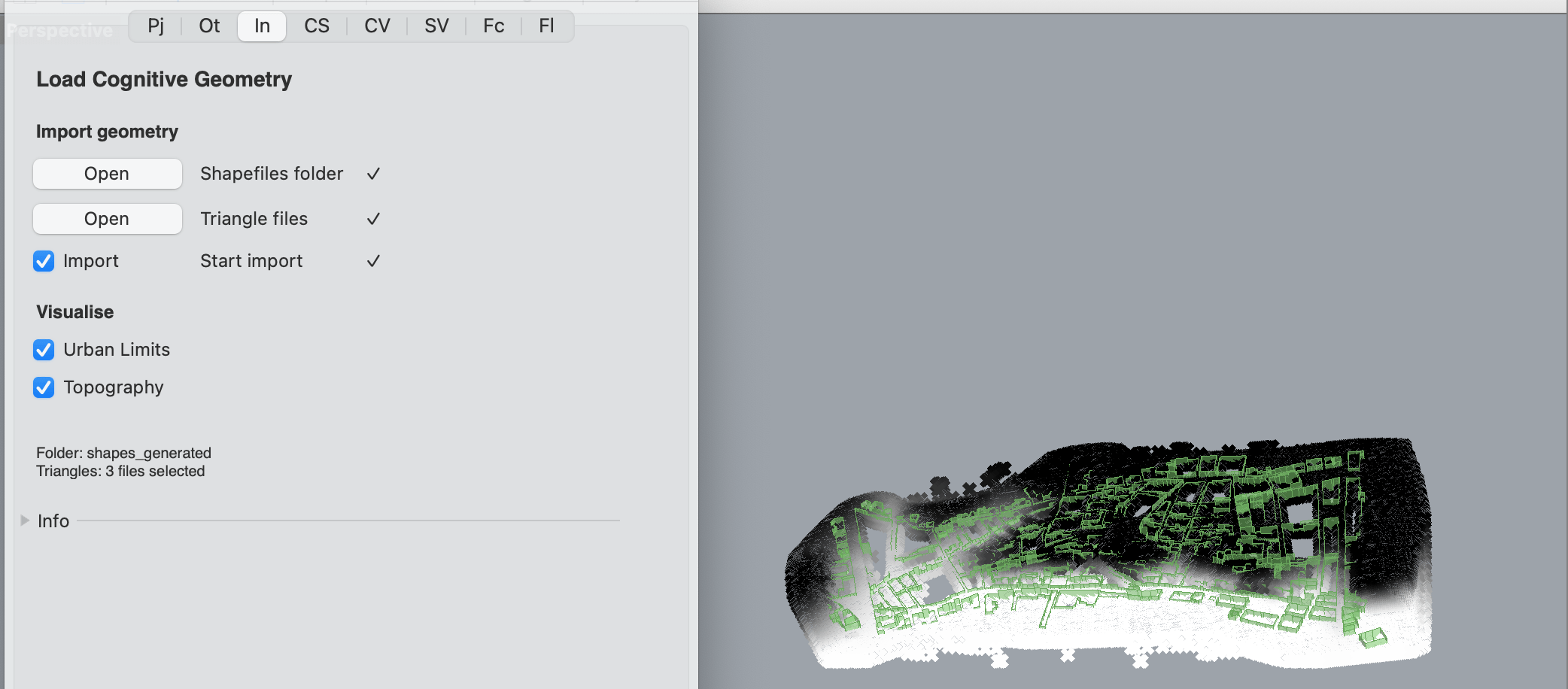
Switch to the In tab and select the folder where the cognitive geometry generated in QGIS was exported. Next, select the trianged mesh within that folder. If the study area is quite large we recommend selecting a limited number of meshes rather than the entire mesh and run the calculations on particular areas first. Click Import and wait for the process to finish.
Once the files have finished importing, you can preview and assess the geometry through the relevant options in the Visualise section of the tab.
2- We can now move on to calculating the Convex Spaces by switching to the CS tab.
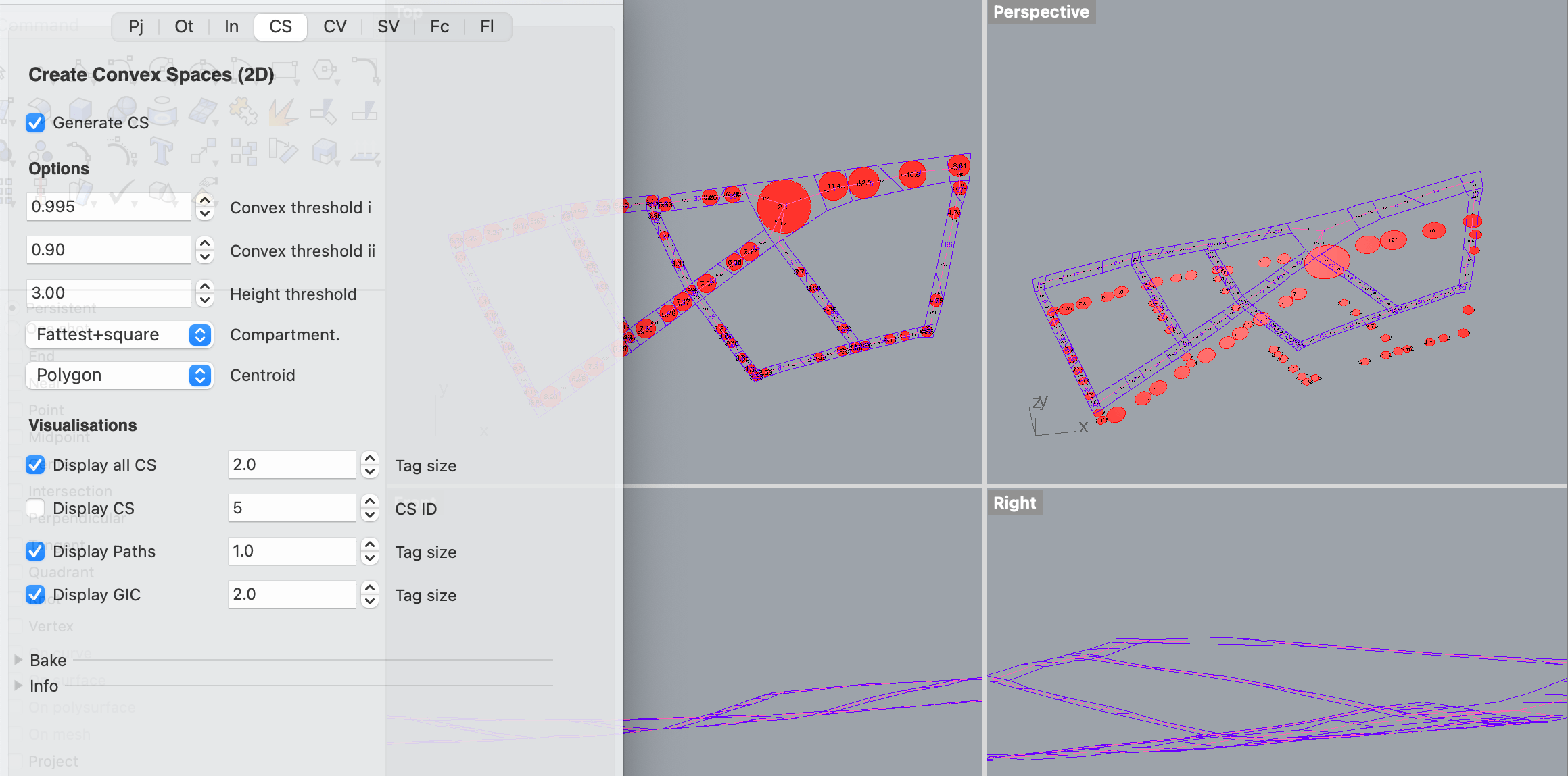
The tab opens with the default options. Whilst we prepare a manual of all the different options, their meanings and definitions can be viewed in the papers published so far. Click on Generate CS to perform the calculation (warning: this is a computationally intensive process that may take some time). Once the calculation is finished, the totality of the convex spaces (CS), individual convex spaces, paths, and greatest inscribed circles (GIC) can be previewed by clicking on the relevant options in the Visualisations section of the tab.
3- The next step involves generating what we term Convex Voids, by switching to the CV tab.
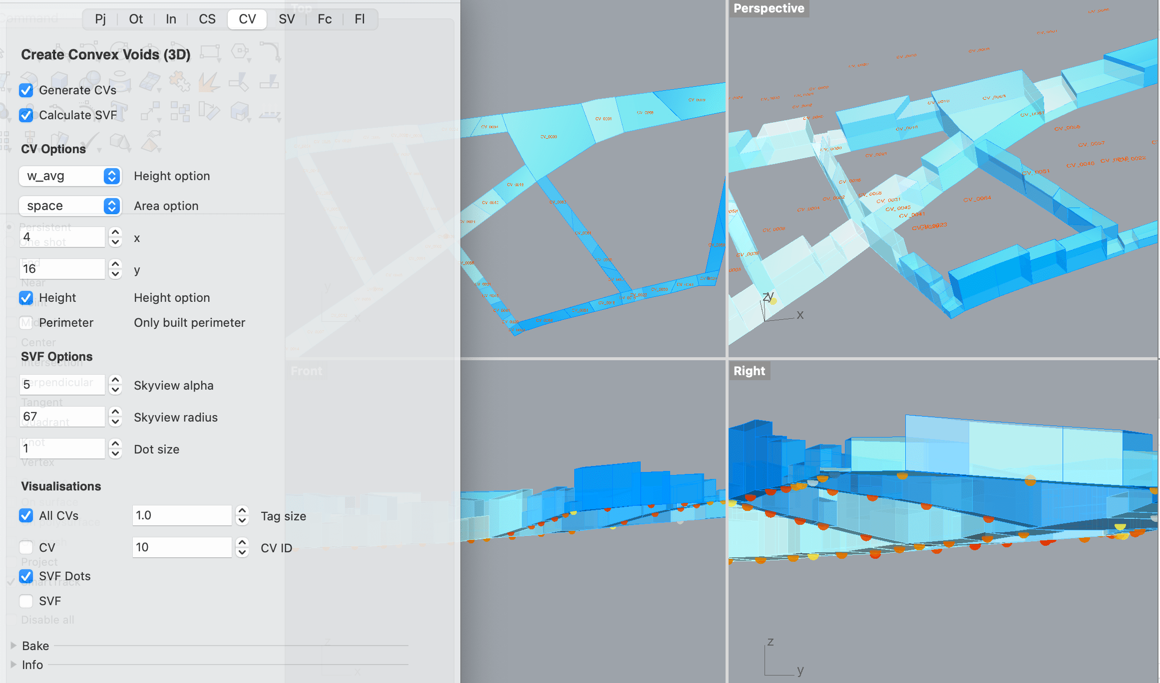
The tab will open with default options. Information on these options can be viewed in the papers published. Make sure the Height option is selected. Click on Generate CVs to proceed with the calculation. Once it finishes, the totality of the convex voids and specific convex voids can be previewed by selecting the relevant options in the Visualisations section of the tab.
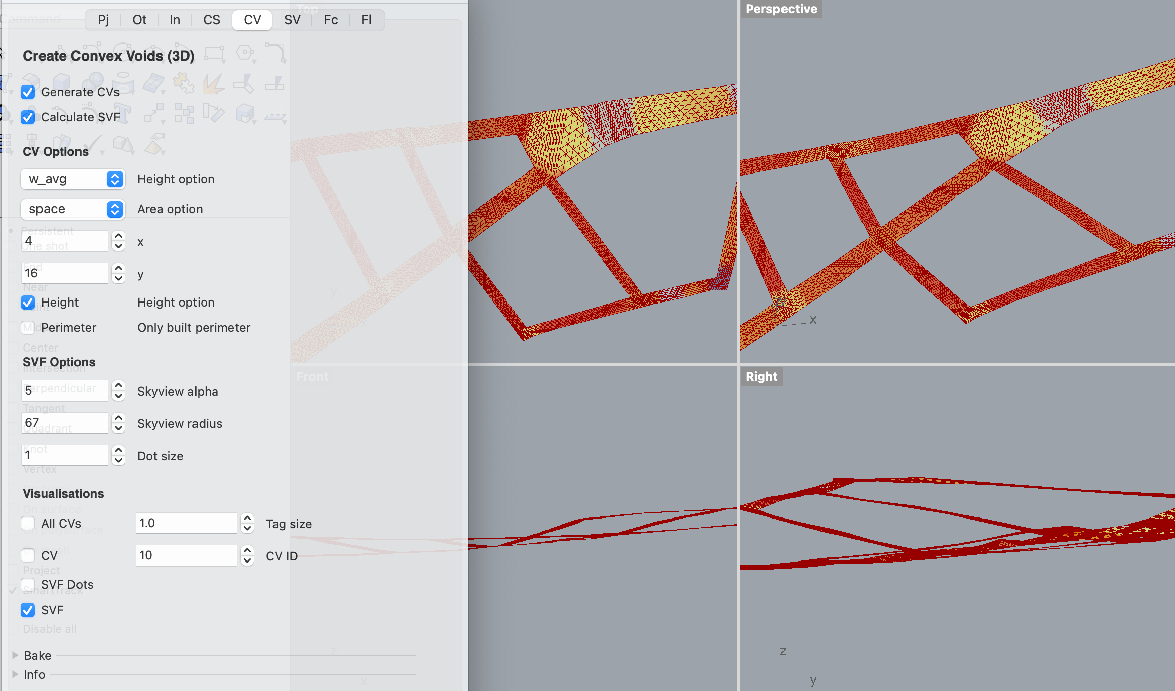
The Sky View Factor (SVF) can also be calculated within this tab. Simply click on Calculate SVF and wait for the process to finish. The output can be previewed by selecting the relevant options within the Visualisations section of the tab.
If you wish, you can expand the Bake section of the tab to bake the previews into permanent Rhino geometry in particular layers. This can also be done for all or particular geometries at the very end of the process by opening the CSV Export window of the Grasshopper panel.
3- The final calculation involves generating what we term Solid Voids (SVs), by switching to the SV tab.
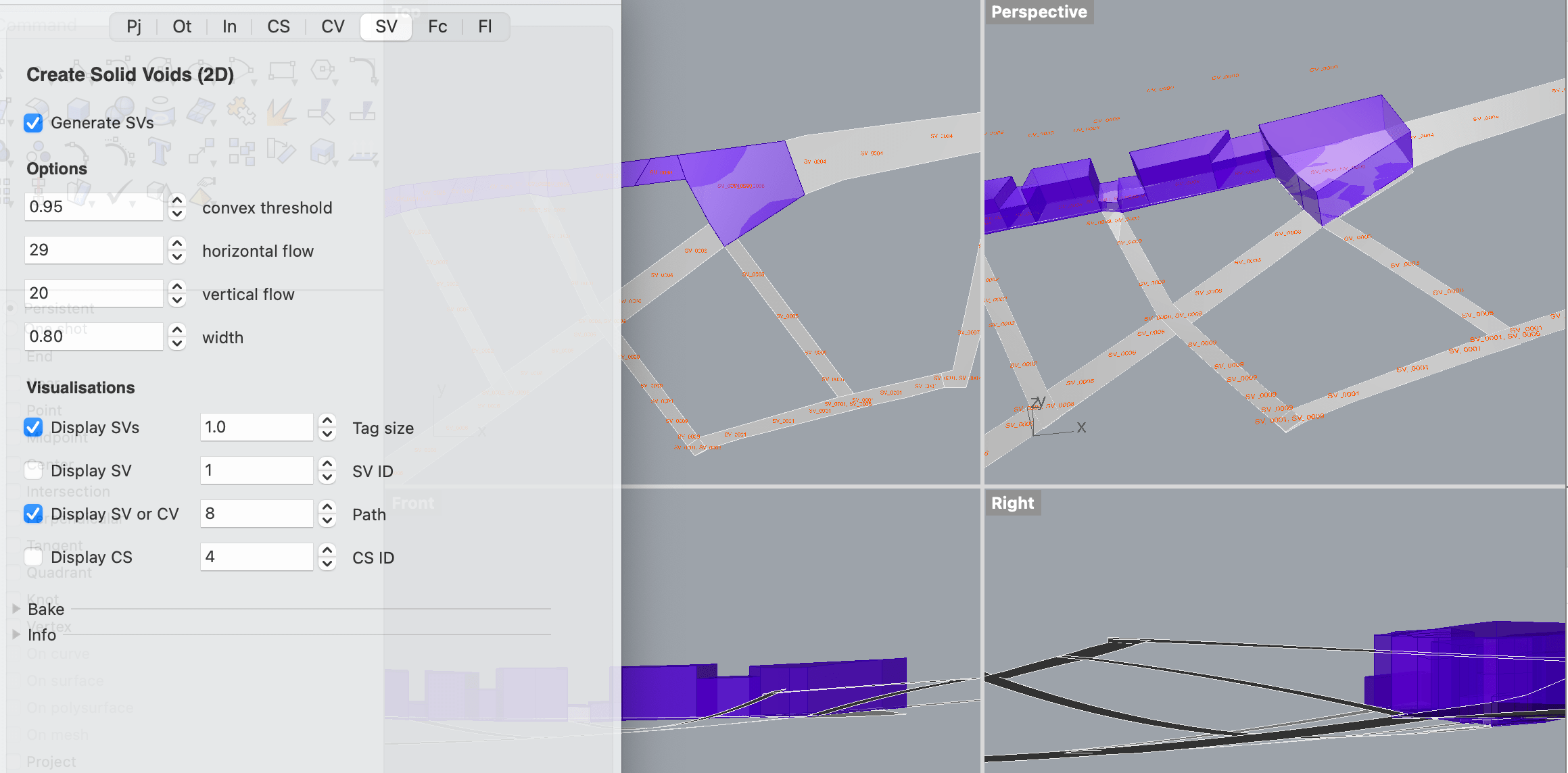
The tab opens with the default options. Information on these options can be viewed in the papers published. Click on Generate SVs to proceed with the calculation and wait for the process to finish.
The totality of the solid voids, particular solid voids, and particular convex voids and convex spaces can be previewed by selecting the relevant options within the Visualisations section of the tab.
If you wish, you can expand the Bake section of the tab to bake the previews into permanent Rhino geometry in particular layers. This can also be done for all or particular geometries at the very end of the process by opening the CSV Export window of the Grasshopper panel.
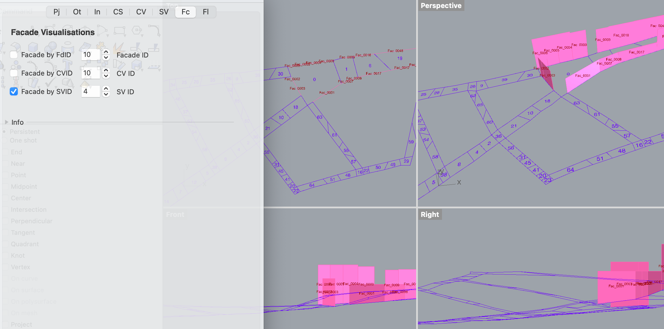
4- Facades and their relation to the voids and convex spaces can be visualised in the Fc tab.
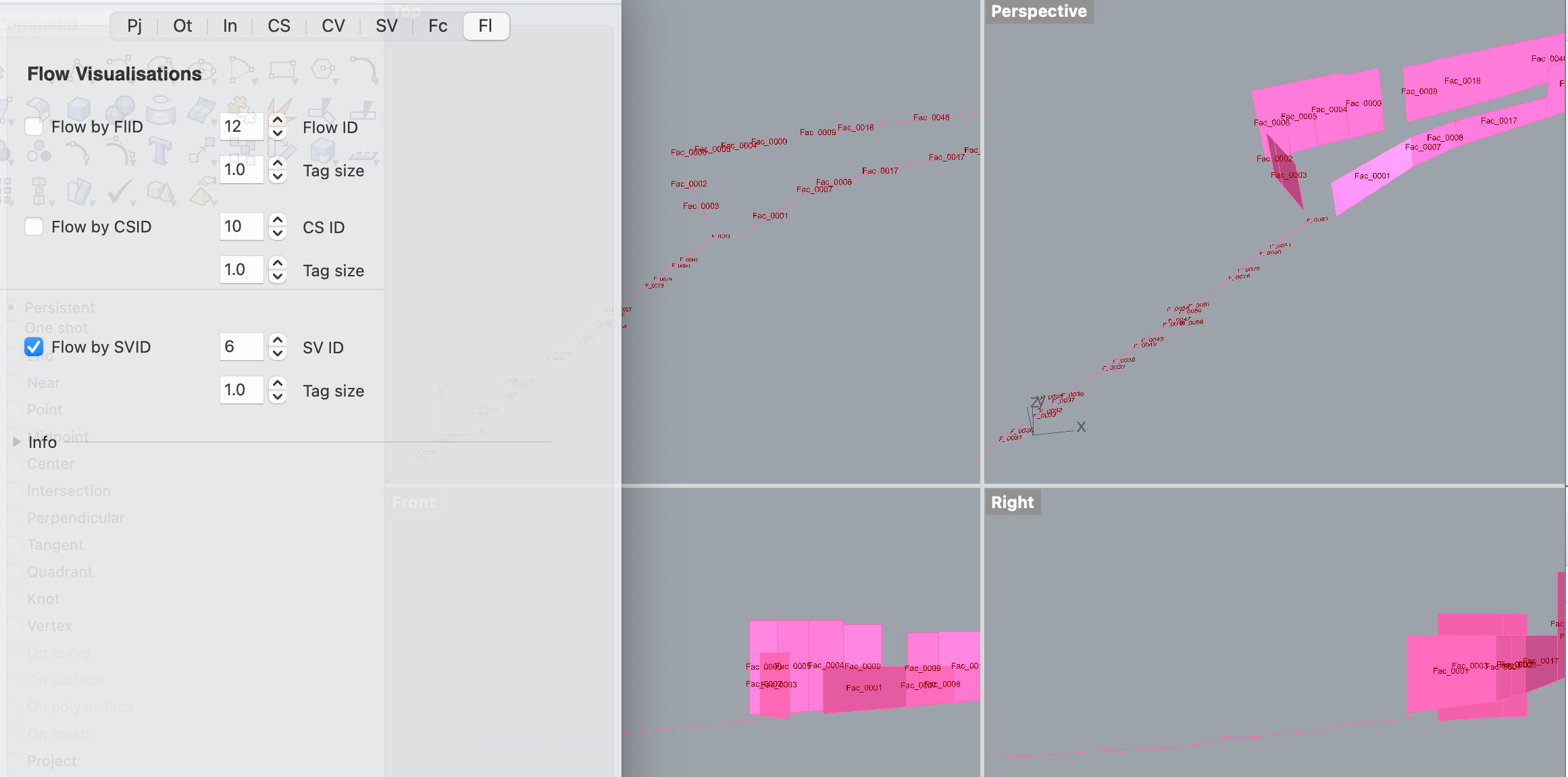
5- Flows and their relation to the voids and convex spaces can be visualised in the Fl tab.
6- Once all the calculations are complete, you can close the CSV Calculate window and open the Export window by clicking on the relevant option in the Grasshopper panel in Rhino.
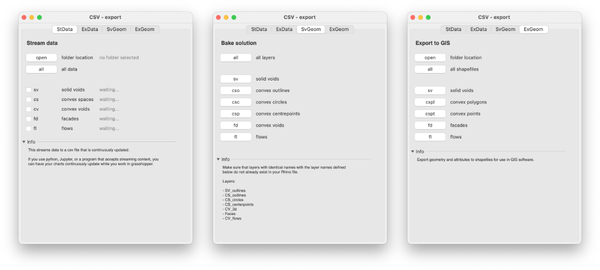
The window is split into four tabs:
- StData (stream data)
- ExData (export data)
- SvGeom (bake solutions)
- ExGeom (export to ESRI shape files)
StData allows you to stream the data generated by the calculations for external real-time analysis. ExData allows you write the final generated data into csv files to import into Excel. SvGeom allows you to bake all or parts of the geometry into the Rhino file. ExGeom allows you to export the geometry and data attributes into shapefiles for use in GIS software.
In the future, we will be providing Jupyter notebooks for real-time analytics and statistical visualisation of the streamed data, as well as integrating a select number of data visualisations within the grasshopper code, allowing you to make changes in any part of the process and have them propagate all the way to the final report building section. Various additional information can be generated using the CS, CV, SV, Facade and Flow data and geometry. Refer to the about page and publications to learn more about the theory and applications of the method.