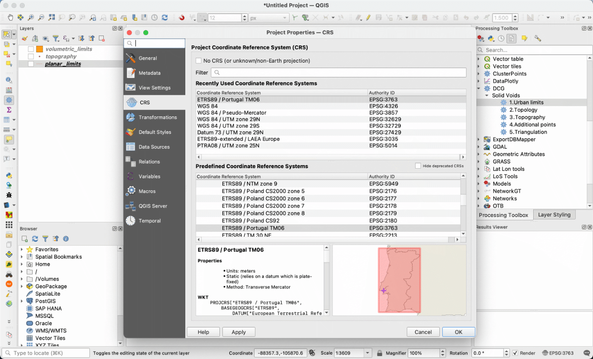
1- Prepare the QGIS working CRS: Always remember to use the correct CRS for your site. For our tutorial, we will be working will Lisbon data which carries the standard Lisbon CRS known as ETRS89 / Portugal TM06 (EPSG:3763). Please make sure QGIS OTF (on the fly transformation) is activated and set to a CRS of EPSG:3763. Whenever you add a file from grasshopper to the project, take a moment to confirm it has the correct CRS. Likewise, whenever you run a script in QGIS, confirm the resulting file has a CRS attached before exporting it. You can define the project CRS by clicking on the bottom right main window globe or by selecting menu item ‘Project -> Properties’. You can define a layer with a known missing CRS through the Processing Toolbox or by right clicking on the layer and selecting ‘Properties’. Do not change the CRS of a layer with a valid coordinate reference system attached (in this case you should re-project it).
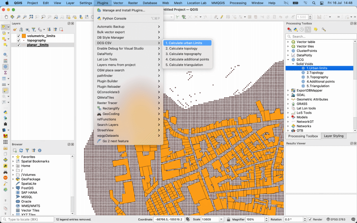
2- Import all shape files generated in the first step to QGIS: volumetric limits, planar limits and topography. The CSV algorithms can be accessed either from the plugins menu, under ‘DCG CSV’, or from the Processing Toolbox, under ‘DCG – Solid Voids’.
3- Run the first code: “Merge Urban Limits.” This code receives volumetric limits and planar limits as input. “There are no horizontal limits” checkbox should be checked at this stage as no horizontal limits are generated in the grasshopper code yet.
Do no assign an output file or directory. Simply let the algorithm save the generated files as temporary layers with their default names for now. We will export them all later. Do the same for all five algorithms. You may leave the settings of all algorithms at their default values (please ignore the values in the screenshots).
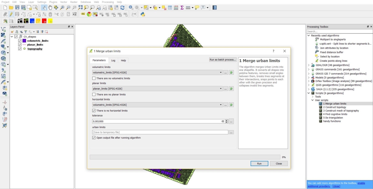
The output of this code will be “urban limits”.
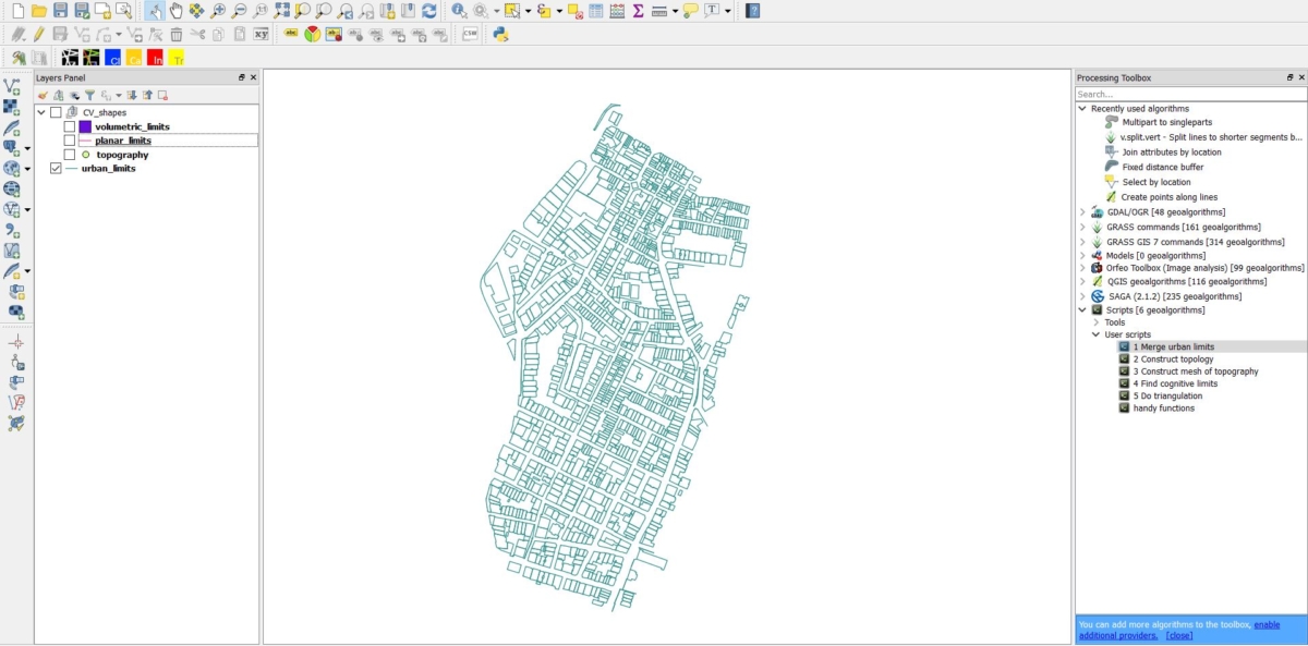
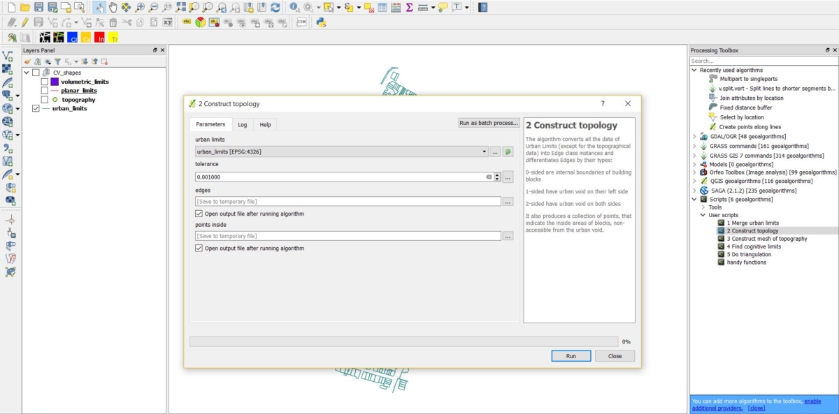
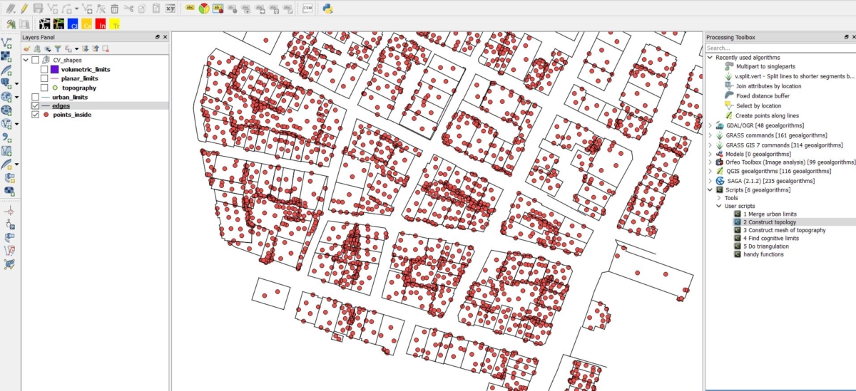
4- Run the second code: “Construct topology.” This code receives “urban limits” as input and creates “points inside” and “edges” as output.
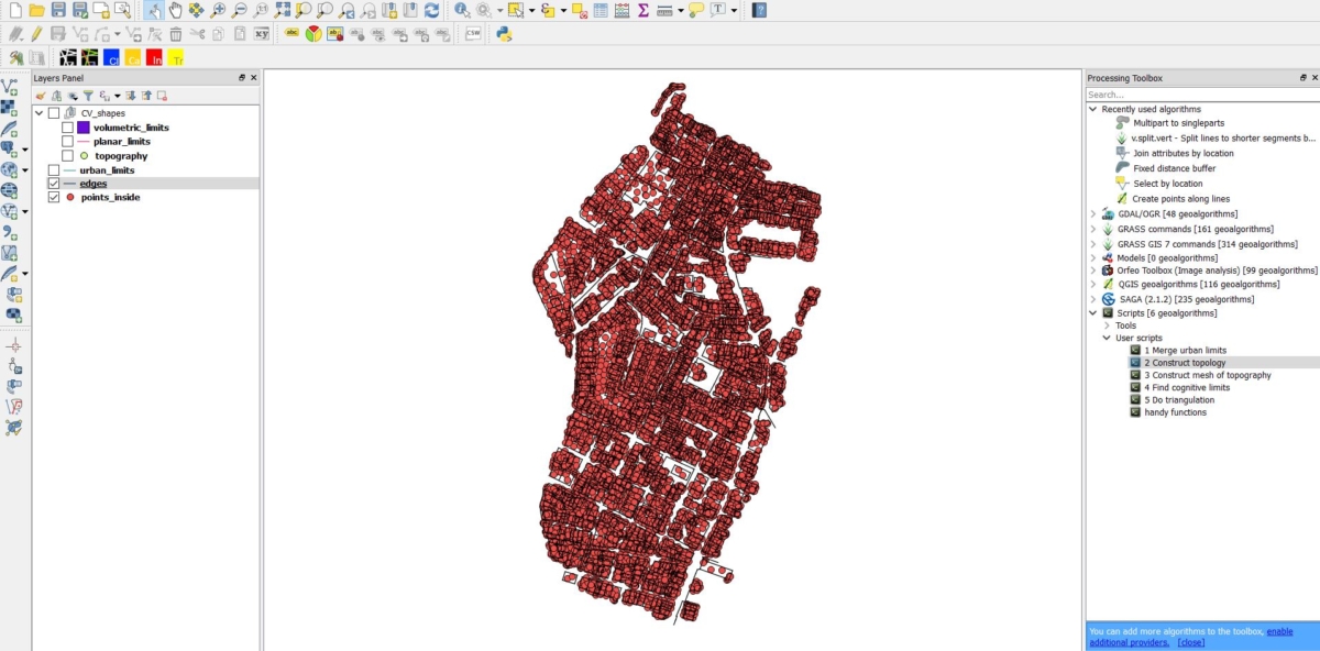
– If you get the error: “not sufficient topography points” do not run the following codes as the final code will not produce geometry after this error. Instead make sure the following issues are resolved and re-run the third code.
- If the topography mesh remains above the upper vertices of any of the urban limits or planar limits at any point, this should be corrected.
- If any geometry extends beyond that of the limits of topography points in plan, the region covered by the topography points should be extended.
- If the error repeats, the topography points may not be dense enough. In this case, a more dense grid of topography points should be generated though extrapolation.
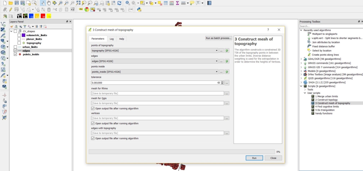
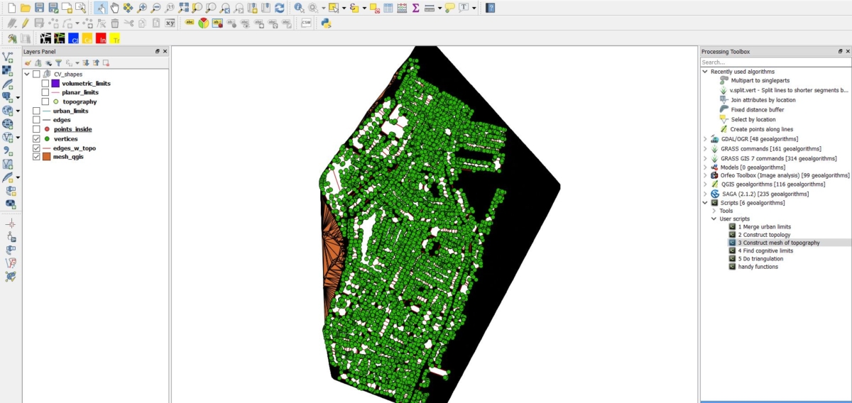
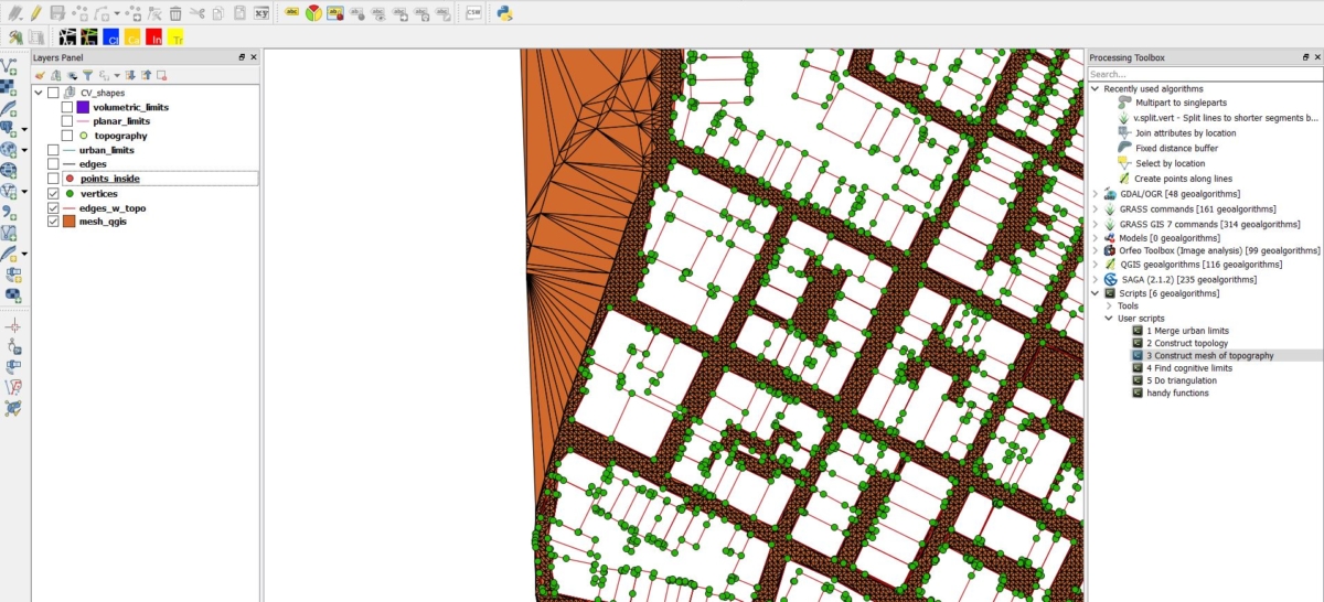
5- Run the third code: “Construct mesh of topography.” This code receives “topography points”, “edges” and “points inside” as input and creates “mesh for qgis”, “vertices”, “edges with topogrpahy.” It also creates a mesh file to be used in the grasshopper code later. This mesh is a .txt file for Rhino. Please save it in your final output folder with the name rhino_mesh.txt.
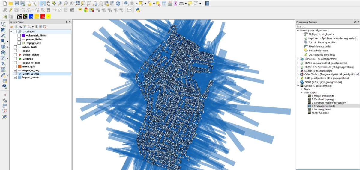
6- Run the fourth code: “Find cognitive limits.” This code receives “edges with topography” and “vertices” as input. The parameters advisable for use for this code are as follows:
- projection parameters: max(LENGTHx15.0,HEIGHTx1.0,UNITSx5.0);;BEARINGorHEIGHTDIFF
- significant vertex bearing: 30.000000
- significant edge height difference per vertex : 3.000000
- tolerance for vertex proximity: 3.000000
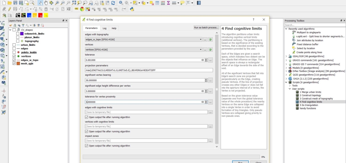
This code defines the implicit limits.
- Search Space: The maximum distance in which implicit points (vertices) should be searched for.
- Attribute of significance: The Significance Precondition of explicit limits to get projected as implicit ones, defined through the bearing angle, vertices’ height difference and vertices minimum horizontal distance.
- When (1) and (2) are satisfied the Explicit limits are projected as Implicit vertices.

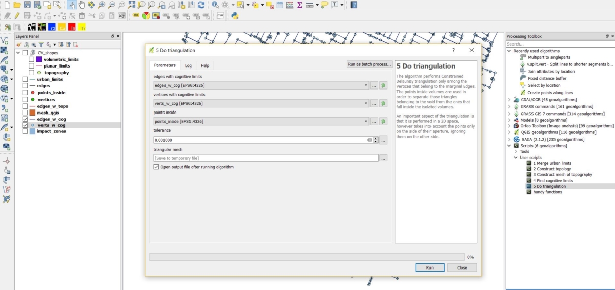
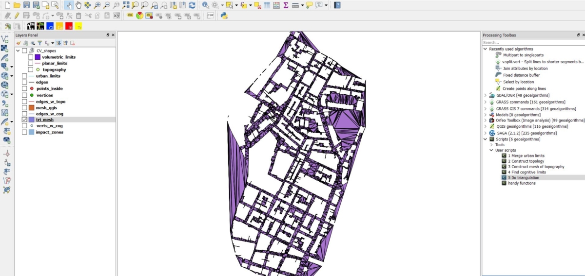
7- Run the fifth code: ” Do triangulation.” This code receives “edges with cognitive limits”, “vertices with cognitive limits” and “points inside” as input and creates the “triangular mesh.”
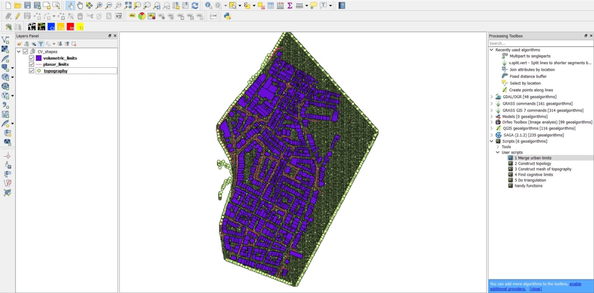
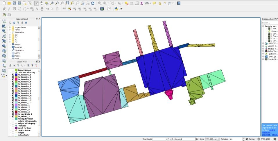
8- Split the mesh: To feed this triangular mesh into the grasshopper definition, it needs to be broken up into smaller meshes. This division needs to be done manually but natural divisible limits of convex spaces should be taken into consideration.
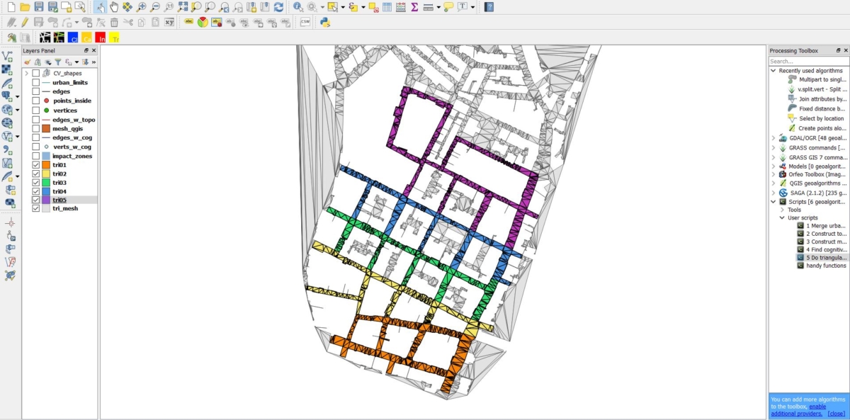
Below is an example demonstrating this division from a different urban context.
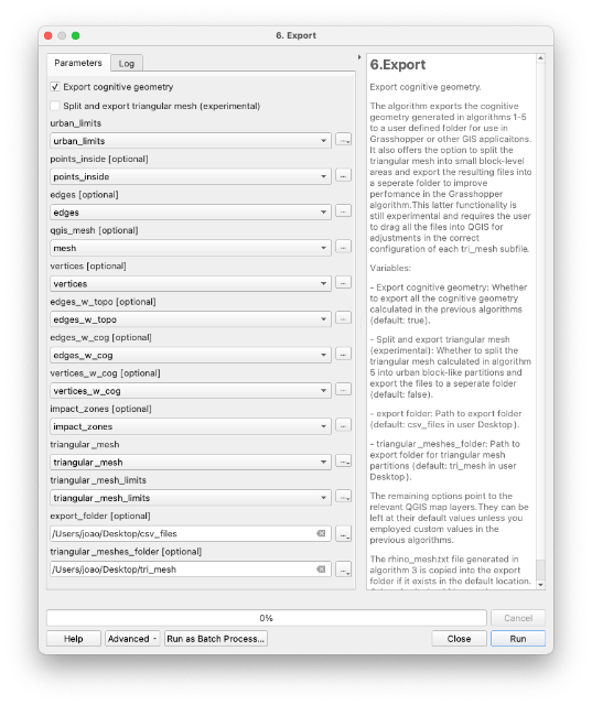
9- Bulk export the layers: Once everything is done, you will have a large number of temporary layers in the layers panel. To save them for future reference and continue the analysis in Rhino, run the sixth code ‘6. Export’. This will export all the layers into shapefiles. You can choose the export location for the files (by default these are placed in a folder on your desktop). The layers are automatically chosen according to their default naming structure – you will need to select them if you used a different structure. If you manually split the triangular mesh, the sub-meshes will all need to be exported as well. You can use a plugin such as ‘bulkvectorexport’ which can export all visible layers in one go. An option is available which will split and export the main triangular mesh – at the moment it is still experimental and we only recommend its usage for the analysis of extremely large urban areas.